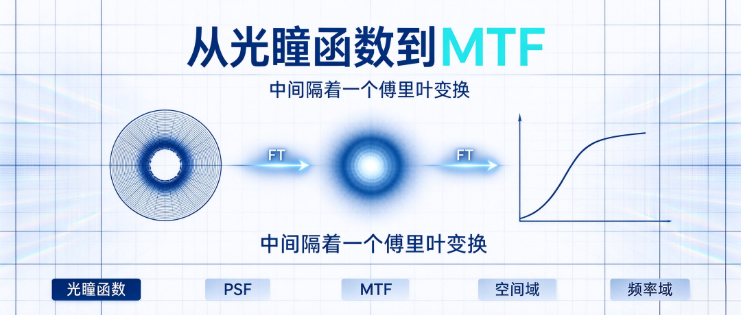
Abstract: The Fourier transform is no mere ornament in optical formulas—it is the underlying mathematical engine that connects the pupil function, PSF, LSF, and MTF. It is what allows the spatial-domain PSF and the frequency-domain MTF to be converted into each other, and what enables the mapping from the pupil function to the PSF. Understanding its role in the evaluation chain matters far more than grinding through mathematical derivations.

For those working in AR optics, the term "Fourier transform" is almost unavoidable. Converting the pupil function to the PSF relies on it; calculating the MTF from the LSF relies on it; simulating Fraunhofer diffraction relies on it; even the sharpening and denoising of AR images rest on the same underlying principle.

Many engineers know how to call this tool but rarely stop to clarify what role the Fourier transform actually plays in an optical system. This article does not pile up complex mathematical derivations—it simply explains where the Fourier transform sits in the optical evaluation chain.

The Essence of the Fourier Transform: Describing the Same Thing in Another Language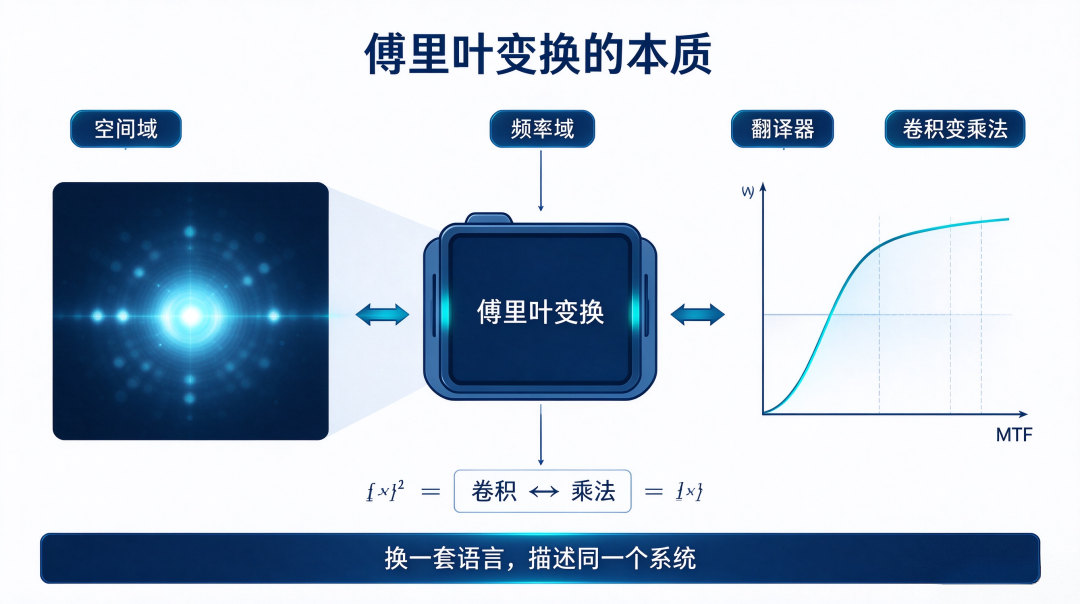

The core idea of the Fourier transform is remarkably simple: any complex signal can be decomposed into a superposition of sine waves at different frequencies.

In the spatial domain, the imaging capability of an optical system is described by the point spread function (PSF): how large a spot an ideal point source will ultimately spread into after passing through the lens.

Switch to the frequency domain, and the imaging capability of the same system is measured by the modulation transfer function (MTF): how much contrast remains after details of varying coarseness in the image pass through the optical system.

The PSF and the MTF describe the same optical system—just in two completely different languages. The Fourier transform is the translator between them.

The complex convolution operation in the spatial domain (convolving the image with the PSF to obtain a blurred image) simplifies directly into a multiplication operation once Fourier-transformed to the frequency domain (image spectrum × MTF). Turning convolution into multiplication is precisely why the Fourier transform can be deployed on such a large scale in optical simulation.

Pupil Function → PSF: The Fourier Transform's First Translation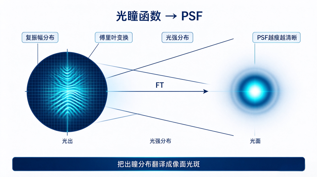

The most fundamental description of an optical system is called the pupil function. It contains two types of information: amplitude information (pupil shape, light transmission capability) and phase information (wavefront error, distortion caused by defocus).

The pupil function is an abstract complex function that cannot be measured directly with instruments. But apply a Fourier transform to it, and you obtain the PSF—a physical quantity that can be measured.

PSF = |FT {pupil function}|

The Fourier transform translates the complex amplitude distribution on the exit pupil plane into the light intensity distribution on the image plane. The more compact the PSF spot and the more concentrated the energy, the higher the imaging clarity. The pupil shape directly determines the PSF form: a circular pupil generates an Airy disk, while an annular pupil yields a finer central spot at the cost of stronger side lobes.

The Fourier transform can accurately calculate this set of geometric correspondences.

PSF → MTF: The Fourier Transform's Second Translation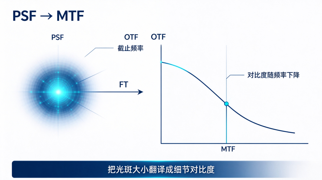

The PSF tells us only one thing: how large a spot a point source will be blurred into. But in engineering, what we care about more is: for image details of varying coarseness, how well does this optical system preserve contrast?

Applying another Fourier transform to the PSF gives the optical transfer function (OTF). The OTF is complex, and taking its modulus yields the familiar MTF.

MTF = |FT{PSF}|

The overall trend of the MTF curve is a gradual decline from low frequency to high frequency: low frequencies correspond to large smooth areas in the image, while high frequencies correspond to fine details such as textures and thin lines. The frequency at which the MTF curve drops to zero is the cutoff frequency of the system.

The core work of the Fourier transform here is to translate "how large a spot a point is blurred into" into "how much contrast remains for details of different fineness"—the former is the PSF, and the latter is the MTF.

Why Can Fraunhofer Diffraction Be Calculated Quickly Using FFT?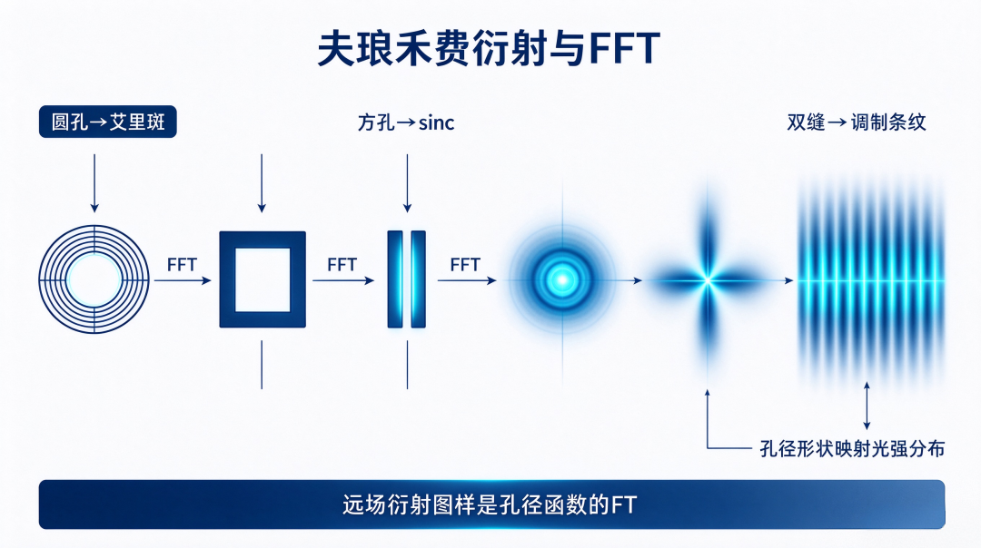

The Fourier transform also has a classic use in optics: simulating Fraunhofer diffraction patterns.

Under Fraunhofer far-field diffraction conditions, the light field distribution of the diffraction spot is exactly equal to the Fourier transform of the aperture function. A circular aperture transforms into an Airy disk (Bessel function); a square aperture produces cross-shaped diffraction fringes corresponding to the sinc function; and double-slit diffraction is the product of two sinc functions, forming modulated equidistant fringes.

The geometric shape of the aperture, after Fourier transformation, maps directly to the light intensity distribution on the observation plane. This is also why, using Python or MATLAB, just a few lines of FFT code can directly simulate the diffraction patterns of circular apertures, square apertures, and double slits.

What Does This Mean for AR Optics Engineers?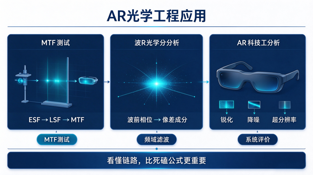

The Fourier transform is not a purely mathematical concept confined to textbooks—it is a tool that AR optics engineers use repeatedly in their daily work.

MTF testing: the edge method collects the ESF, differentiation gives the LSF, and then a Fourier transform is performed to calculate the MTF.

Wavefront analysis: the interferometer measures the wavefront phase, and the Fourier transform is used to decompose the various aberration components.

Image processing: the sharpening, denoising, and super-resolution algorithms in AR glasses are all based on frequency-domain filtering.

Understanding the role of the Fourier transform in the optical chain is more important than grinding through complex mathematical derivations. The former helps you judge when to use it; the latter only solves how to calculate it.

Conclusion

From the pupil function to the PSF, from the PSF to the MTF, from aperture shape to diffraction pattern, the Fourier transform is the underlying engine running through the entire AR optical evaluation system.

It is not a decorative term added to formulas for embellishment, but a translator that connects the spatial domain and the frequency domain. Only by understanding the role of this translator can one fully grasp the underlying logic of optical system evaluation.

Interactive topic: In your AR optics work, where does the Fourier transform most often appear—MTF calculation, wavefront analysis, or image processing? You are welcome to leave a message and share your experience.

[Risk note] This article is a popular science piece on optical engineering. The Fourier transform, PSF, and MTF described herein are general principles; actual optical systems will have coupled effects such as aberrations, defocus, and noise, and simulation results will deviate from actual measurements. System performance is ultimately subject to the measured data of the complete machine. — AR Andy | Focused on the optical waveguide and AR microdisplay track, providing in-depth analysis of the underlying logic of the optical industry