Analysis: The Future of AI Generation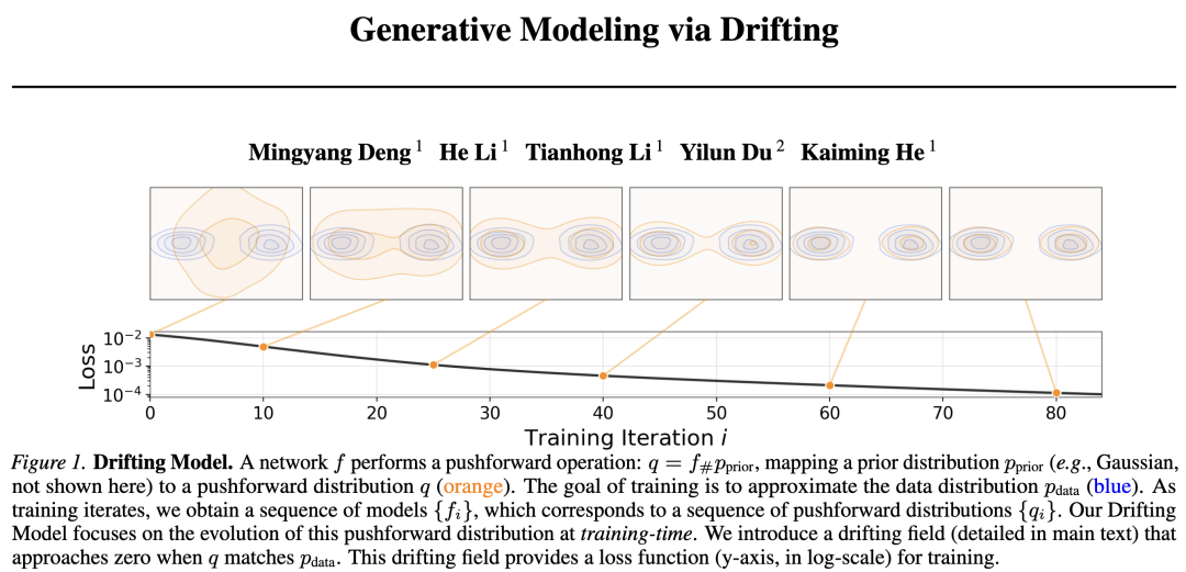

Key Highlights

A New Generative Paradigm: Introduces 'Drifting Models,' a paradigm that eliminates the need for iterative inference by shifting the distribution evolution process to the training phase.

True One-Step Generation: Achieves high-quality one-step (One-step / 1-NFE) generation without distillation, fundamentally addressing the slow inference speed of diffusion models.

SOTA Performance: On ImageNet, one-step generation achieves an FID of 1.54, outperforming all existing one-step methods and even rivaling multi-step diffusion models.

Universal Drift Field Theory: Introduces a physics-inspired 'drift field' concept that drives the model to equilibrium by minimizing sample drift.

Problems Solved

Inference Efficiency Bottleneck: Existing diffusion and flow matching models rely on iterative denoising during inference (e.g., 20-100 steps), leading to slow generation and high computational costs.

Insufficient Quality in One-Step Generation: While one-step methods like Consistency Models exist, they often require complex distillation processes and struggle to match the quality of multi-step models.

Training-Inference Misalignment: Traditional methods simulate dynamic evolution during inference, whereas this work achieves distribution evolution through iterative optimization during training, simplifying inference to a single mapping.

Proposed Solution

Training-Time Evolution: Leverages the iterative nature of deep learning training (e.g., SGD steps) to evolve pushforward distributions with each parameter update.

Drift Field: Defines a vector field that describes how generated samples should move to approximate the data distribution. This field is determined by the attraction of the data distribution and the repulsion of the current generated distribution.

Equilibrium Training Objective: Constructs a loss function aimed at minimizing the magnitude of the drift field. When the generated distribution matches the data distribution (), the drift field becomes zero, achieving equilibrium.

Feature Space Manipulation: For better training signals, drift field calculations are performed in a pretrained feature space (e.g., Latent-MAE) rather than directly in pixel space.

Technologies Applied

Pushforward Distribution: Models the generative process using .

Kernel Density Estimation and Mean Shift: Uses kernel functions to estimate interaction forces between samples, simulating particle motion in a field.

Contrastive Learning: Estimates the drift field using positive samples (real data) and negative samples (generated data), similar to positive-negative pairs in contrastive learning.

Latent-MAE: Trains an MAE model operating in latent space as a feature extractor to support generation in both pixel and latent spaces.

Achieved Results

ImageNet 256×256:

Latent Space: FID 1.54 (1-NFE), outperforming SiT-XL/2 (2.06) and DiT-XL/2 (2.27).

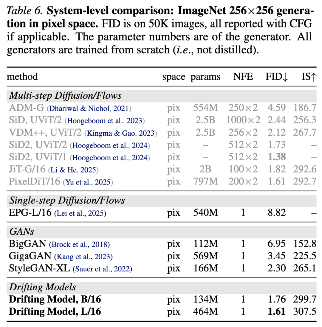
Pixel Space: FID 1.61 (1-NFE), significantly outperforming StyleGAN-XL (2.30) and ADM (4.59).

Robot Control: On the Diffusion Policy benchmark, achieves success rates comparable to or better than 100-NFE diffusion policies with just 1-NFE inference.

CFG-Free: Best performance achieved at CFG scale = 1.0, eliminating the need for additional classifier-free guidance computation.

Generative modeling is generally considered more challenging than discriminative modeling. Discriminative modeling focuses on mapping individual samples to their corresponding labels, whereas generative modeling involves mapping from one distribution to another. This can be formulated as learning a mapping such that the pushforward distribution of a prior distribution matches the data distribution, i.e., . Conceptually, generative modeling learns a functional (here, ), which maps one function (here, a distribution) to another.

This 'pushforward' behavior can be realized iteratively during inference, as seen in popular paradigms like diffusion models (Diffusion) (Sohl-Dickstein et al., 2015) and flow matching (Flow Matching) (Lipman et al., 2022). During generation, these models map noisier samples to slightly cleaner ones, gradually evolving the sample distribution toward the data distribution. This modeling philosophy can be viewed as decomposing a complex pushforward mapping (i.e., ) into a series of feasible transformations applied during inference.

In this paper, we introduce Drifting Models, a new paradigm for generative modeling. Drifting Models are characterized by learning a pushforward mapping that evolves during training, eliminating the need for iterative inference. The mapping is represented by a single-pass, non-iterative network. Since the training process in deep learning optimization is inherently iterative, this can naturally be viewed as evolving the pushforward distribution by updating . See Figure 1 above.

To drive the evolution of the pushforward distribution during training, we introduce a drift field that governs sample movement. This field depends on both the generated distribution and the data distribution. By definition, when the two distributions match, the field becomes zero, achieving an equilibrium state where samples no longer drift.

Based on this concept, we propose a simple training objective to minimize the drift of generated samples. This objective induces sample movement and evolves the underlying pushforward distribution through iterative optimization (e.g., SGD). We further introduce the design of the drift field, neural network model, and training algorithm.

Drifting Models naturally perform one-step ('1-NFE') generation and achieve strong empirical performance. On ImageNet, we obtain a 1-NFE FID of 1.54 under the standard latent space generation protocol, setting a new state-of-the-art among one-step methods. This result remains competitive even when compared to multi-step diffusion/flow models. Additionally, under the more challenging pixel space generation protocol (i.e., without latents), we achieve a 1-NFE FID of 1.61, significantly outperforming previous pixel space methods. These results demonstrate that Drifting Models provide a promising new paradigm for high-quality, efficient generative modeling.

Related Work

Diffusion/Flow-based Models. Diffusion models and their flow-based counterparts formulate the noise-to-data mapping via differential equations (SDEs or ODEs). The core of their inference-time computation involves iterative updates, e.g., in the form of , using solvers like Euler. Updating relies on a neural network , so generation involves multi-step network evaluations.

Increasing efforts focus on reducing steps in diffusion/flow models. Distillation-based methods distill pretrained multi-step models into one-step models. Another line of research aims to train one-step diffusion/flow models from scratch. To achieve this, these methods incorporate SDE/ODE dynamics into training by approximating induced trajectories. In contrast, our work proposes a conceptually different paradigm and does not rely on SDE/ODE formulations like diffusion/flow models.

Generative Adversarial Networks (GANs). GANs are a classic family of generative models that train a generator by distinguishing generated samples from real data. Like GANs, our method involves a single-pass network that maps noise to data, with its 'goodness' evaluated by a loss function; however, unlike GANs, our method does not rely on adversarial optimization.

Variational Autoencoders (VAEs). VAEs optimize the Evidence Lower Bound (ELBO), which includes a reconstruction loss and a KL divergence term. Classical VAEs are one-step generators when using a Gaussian prior. Today's popular VAE applications often resort to priors learned from other methods, such as diffusion or autoregressive models, where the VAE effectively serves as a tokenizer.

Normalizing Flows. NFs learn a mapping from data to noise and optimize sample log-likelihood. These methods require invertible architectures and computable Jacobian determinants. Conceptually, NFs operate as one-step generators during inference, with computation performed by the network's inverse.

Moment Matching. Moment matching methods seek to minimize the Maximum Mean Discrepancy (MMD) between generated and data distributions. Moment matching has recently been extended to one-step/few-step diffusion. Related to MMD, our method also leverages kernel functions and the concept of positive/negative samples. However, our method focuses on a drift field that explicitly controls sample drift during training.

Contrastive Learning. The drift field in our work is driven by positive samples from the data distribution and negative samples from the generated distribution. This is conceptually related to positive-negative pairs in contrastive representation learning. The idea of contrastive learning has also been extended to generative models, such as GANs or Flow Matching.

Drifting Models for Generation

This paper introduces Drifting Models, which formulate generative modeling as the training-time evolution of pushforward distributions via a drift field. Our model naturally performs one-step generation during inference.

Training-Time Pushforward

Consider a neural network . The input to is (e.g., noise of arbitrary dimension ), and the output is denoted as . Typically, the input and output dimensions need not be equal.

We use to denote the distribution of the network's output, i.e., . In probability theory, is called the pushforward distribution of under , denoted as:

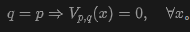
Here, ' ' denotes the pushforward induced by . Intuitively, this notation means that transforms distribution into another distribution . The goal of generative modeling is to find such that .

Since neural network training is inherently iterative (e.g., SGD), the training process produces a sequence of models , where denotes the training iteration. This corresponds to a sequence of pushforward distributions during training, where for each , . The training process gradually evolves to match .

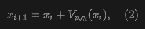
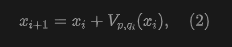
When network updates, samples at training iteration implicitly 'drift' to: , where arises from the parameter update to . This means that the update to determines the 'residual' of , which we refer to as the 'drift' (drift).

Drift Field for Training

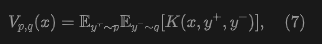
Next, we define a drift field to control the training-time evolution of samples and, consequently, the pushforward distribution . The drift field is a function that computes given . Formally, denoting the field as , we have:

Here, , and the drift is denoted as . The subscript indicates that the field depends on (e.g., ) and the current distribution .

Ideally, when , we want all to stop drifting, i.e., . Consider the following proposition:

Proposition 3.1. Consider an anti-symmetric drift field:

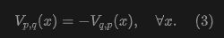
Then we have:

The proof is straightforward. Intuitively, anti-symmetry means that swapping and simply flips the sign of the drift. This proposition implies that if the pushforward distribution matches the data distribution , then for any sample, the drift is zero, and the model achieves equilibrium.

Note that the converse (i.e., ) does not generally hold for an arbitrarily chosen . For our kernelized formulation, we provide sufficient conditions under which implies .

Training Objective. The equilibrium property motivates the definition of the training objective. Let be a network parameterized by , where . At the equilibrium point of , we establish the following fixed-point relationship:

Here, denotes the optimal parameters that achieve equilibrium, and denotes the pushforward distribution of .

This equation motivates fixed-point iteration during training. At iteration , we seek to satisfy:

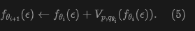
We convert this update rule into a loss function:

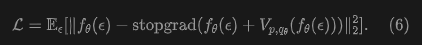
Here, the stop-gradient operation provides a frozen state from the previous iteration. Intuitively, we compute a frozen target and move the network prediction toward it.

We note that the value of the loss function equals , i.e., the squared norm of the drift field . Through the stop-gradient formulation, our solver does not directly backpropagate through , as depends on , and backpropagating through distributions is highly challenging. Instead, our formulation minimizes the objective indirectly: it moves toward its drifted version, i.e., toward the frozen at that iteration.

Drift Field Design

The field depends on two distributions and . To obtain a computable formula, this paper considers the following form:

Here, is a kernel-like function describing the interaction among three sample points. may optionally depend on and . The framework in this paper supports a broad class of functions , as long as when .

For the instantiation in this paper, a form of driven by attraction and repulsion is introduced. Inspired by the mean-shift method (Cheng, 1995), this paper defines the following field:

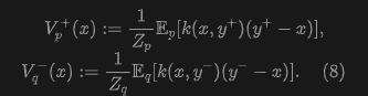
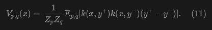
Here, and are normalization factors:

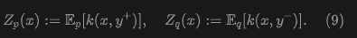
Intuitively, formula (8) computes a weighted average of the vector differences . The weights are given by the kernel and normalized by (9). This paper then defines as:

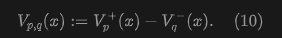
Intuitively, this field can be seen as being attracted by the data distribution and repelled by the sample distribution , as shown in Figure 2.

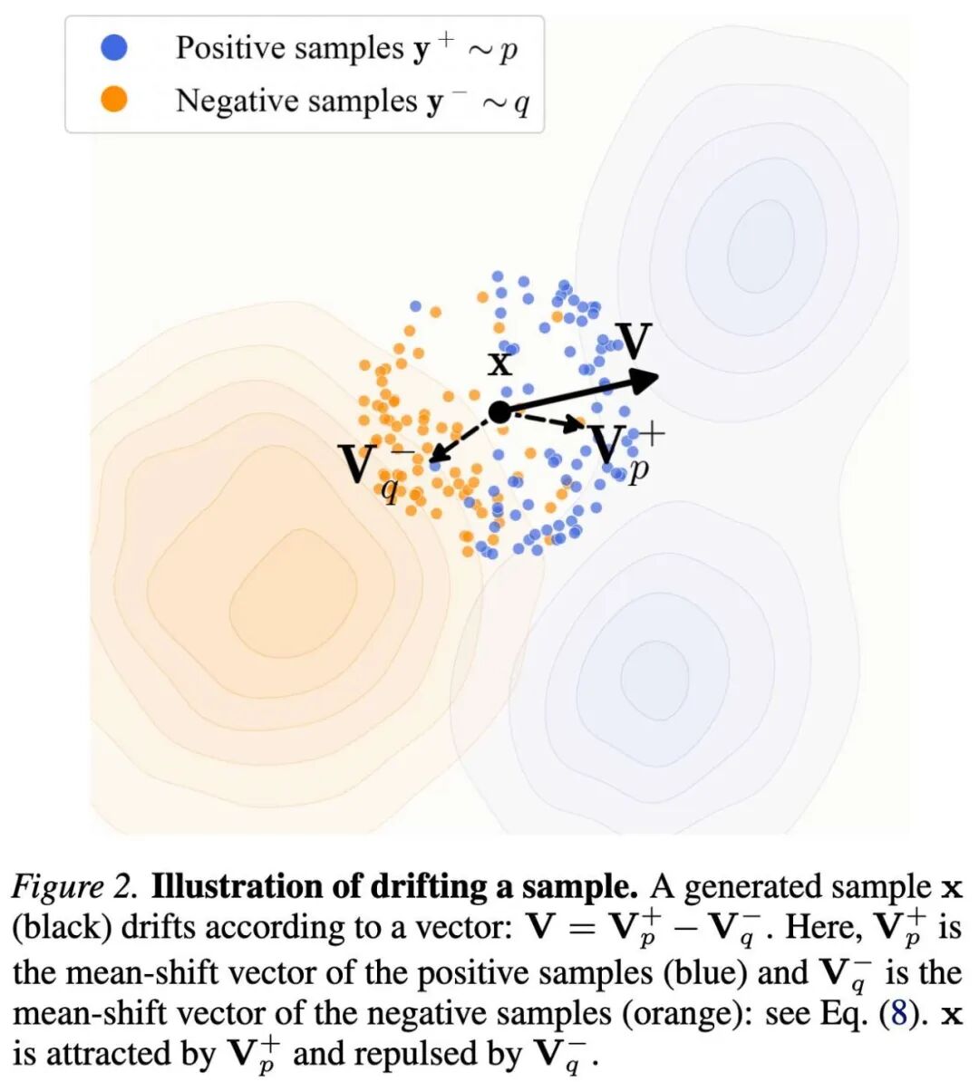Figure 2. Schematic of drifting samples. Generated samples (black) drift according to the vector . Here, is the mean-shift vector for positive samples (blue), and is the mean-shift vector for negative samples (orange): see formula (8). is attracted by and repelled by .

Substituting formula (8) into formula (10), this paper obtains:

Here, the vector difference simplifies to ; the weights are computed by two kernels and jointly normalized. This form is an instantiation of formula (7). It is easy to see that is antisymmetric: . In general, this paper's method does not require decomposing into attraction and repulsion; it only requires that when .

Kernel Function (Kernel). The kernel can be a function measuring similarity. In this paper, this paper adopts:

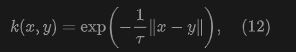
where is the temperature, and is the -distance. This paper views as a normalized kernel, which absorbs the normalization in formula (11).

In practice, the softmax operation is used to implement , where logits are given by , and softmax is performed over . This softmax operation is similar to InfoNCE in contrastive learning. In this paper's implementation, this paper further applies an additional softmax normalization over the set of within a batch, which slightly improves performance in practice. This additional normalization does not alter the antisymmetric property of the resulting .

Balancing and Matching Distributions. Since this paper's training loss in formula (6) encourages minimizing , this paper hopes that leads to . While this implication does not hold for arbitrarily chosen , this paper empirically observes that reducing the value of correlates with improved generation quality. In Appendix C.1, this paper provides an identifiability heuristic argument: for this paper's kernelized construction, the zero-drift condition imposes a large number of bilinear constraints on , which, under mild non-degeneracy assumptions, enforces and to (approximately) match.

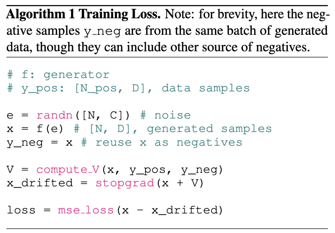
Stochastic Training. In stochastic training (e.g., mini-batch optimization), this paper estimates by approximating the expectation in formula (11) with empirical means. For each training step, this paper draws noise samples and computes a batch of . Generated samples are also used as negative samples within the same batch, i.e., . On the other hand, this paper samples data points . The drift field is computed over this batch of positive and negative samples. Algorithm 1 provides pseudocode for such a training step, where compute V is given in Section A.1.

Drifting in Feature Space

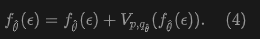
So far, this paper has directly defined the objective (6) in the original data space. This paper's formulation can be extended to any feature space. Let denote a feature extractor (e.g., an image encoder) operating on real or generated samples. This paper rewrites the loss (6) in feature space as:

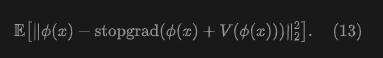
Here, is the generator's output (e.g., an image). is defined in feature space: in practice, this means and serve as positive/negative samples. Notably, feature encoding is a training-time operation and is not used during inference.

This can be further extended to multiple features, e.g., at multiple scales and positions:

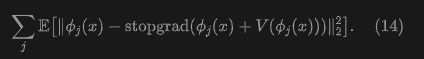
Here, denotes the feature vector from encoder at the -th scale and/or position. Using a ResNet-style image encoder, this paper computes the drift loss at multiple scales and positions, providing richer gradient information for training.

The feature extractor plays an important role in high-dimensional data generation. Since this paper's method characterizes sample similarity based on the kernel , it is desirable for semantically similar samples to remain close in feature space. This goal aligns with self-supervised learning. This paper uses pre-trained self-supervised models as feature extractors.

Relation to Perceptual Loss. This paper's feature space loss is related to but conceptually distinct from perceptual loss (Zhang et al., 2018). Perceptual loss minimizes: , i.e., the regression target is and requires pairing with its target. In contrast, this paper's regression target in (13) is , where the drift is in feature space and no pairing is required. In principle, this paper's feature space loss aims to match the pushed-forward distributions and .

Relation to Latent Generation. This paper's feature space loss is orthogonal to the concept of generators in latent space (e.g., Latent Diffusion). In this paper's case, when using , the generator can still produce output in the pixel space or latent space of the tokenizer. If the generator operates in latent space and the feature extractor in pixel space, a tokenizer decoder will be applied before extracting features from .

Classifier-Free Guidance

Classifier-Free Guidance (CFG) improves generation quality by extrapolating between class-conditional and unconditional distributions. This paper's method naturally supports a related form of guidance.

In this paper's model, given a class label as a condition, the underlying target distribution now becomes , from which positive samples can be drawn: . To achieve guidance, this paper draws negative samples from generated samples or real samples of different classes. Formally, the negative sample distribution is now:

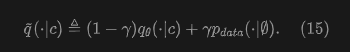
Here, is the mixing rate, and denotes the unconditional data distribution (Footnote 2: This should be the data distribution excluding class . For simplicity, this paper uses the unconditional data distribution).

The learning objective is to find . Substituting it into (15), this paper obtains:

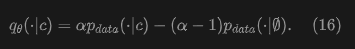
where . This means is to approximate a linear combination of the conditional and unconditional data distributions. This follows the spirit of the original CFG.

In practice, formula (15) means that in addition to generated data, this paper samples additional negative samples from data in . The distribution corresponds to a class-conditional network , similar to common practice. This paper notes that in this paper's method, CFG is a training-time behavior by design: the one-step (1-NFE) property is preserved at inference time.

Implementation for Image Generation

This paper describes the implementation of image generation on ImageNet at resolution .

Tokenizer. By default, this paper performs generation in latent space. This paper adopts the standard SD-VAE tokenizer, which produces a latent space where generation occurs.

Architecture. This paper's generator () has an architecture similar to DiT (Peebles & Xie, 2023). Its input is -dimensional Gaussian noise , and its output is generated latent of the same dimension. This paper uses a patch size of 2, i.e., like DiT/2. This paper's model uses adaLN-zero to handle class conditioning or other additional conditions.

CFG Conditioning. This paper adopts CFG conditioning. During training, a CFG scale (formula 16) is randomly sampled. Negative samples are prepared according to (formula 15), and the network is conditioned on this value. At inference time, can be freely specified and varied without retraining.

Batching. The pseudocode in Algorithm 1 describes a batch of generated samples. In practice, when class labels are involved, this paper samples a batch of class labels. For each label, this paper independently executes Algorithm 1. Thus, the effective batch size is , consisting of negative samples and positive samples.

This paper defines a "training epoch" based on the number of generated samples . Specifically, samples are generated per iteration, and for a dataset of size , one epoch corresponds to iterations.

Feature Extractor. This paper's model trains the drift loss in feature space. The feature extractor is an image encoder. This paper mainly considers ResNet-style

encoders, e.g., those pre-trained with self-supervised learning such as MoCo and SimCLR. When these pre-trained models operate in pixel space, this paper applies a VAE decoder to map the generator's latent space output back to pixel space for feature extraction. Gradients are backpropagated through the feature encoder and VAE decoder. This paper also studies MAE pre-trained in latent space.

For all ResNet-style models, features are extracted from multiple stages (i.e., multi-scale feature maps). The drift loss (13) is computed at each scale and then combined.

Pixel Space Generation. While this paper's experiments mainly focus on latent space generation, this paper's model supports pixel space generation. In this case, both and are . This paper uses a patch size of 16 (i.e., DiT/16). The feature extractor operates directly on pixel space.

Experiments

Toy Experiments

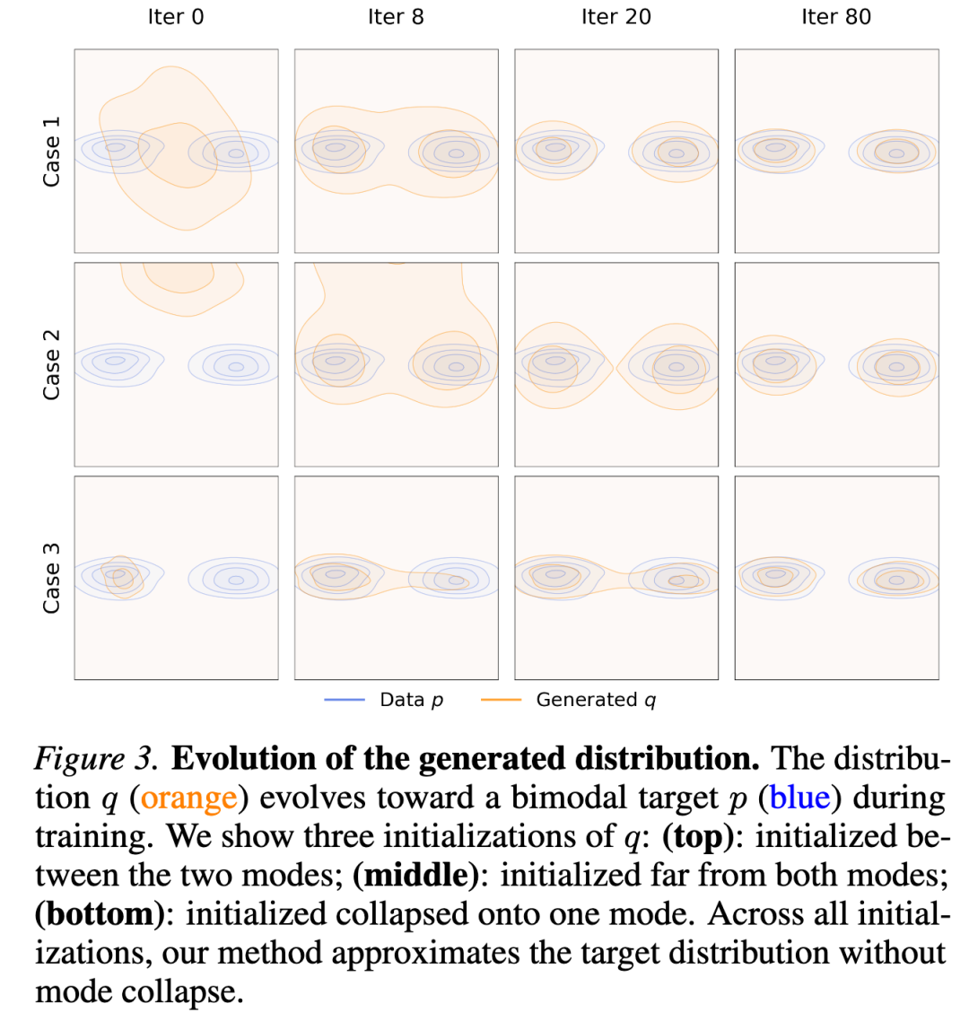
Evolution of Generated Distributions. Figure 3 visualizes a 2D case where evolves toward a bimodal distribution during training under three initializations. In this example, this paper's method approximates the target distribution without exhibiting mode collapse. This holds even when is initialized in a collapsed unimodal state (bottom). This provides an intuitive explanation for why this paper's method is robust to mode collapse: if collapses onto one mode, the other modes in will attract samples, allowing them to continue moving and push to keep evolving.

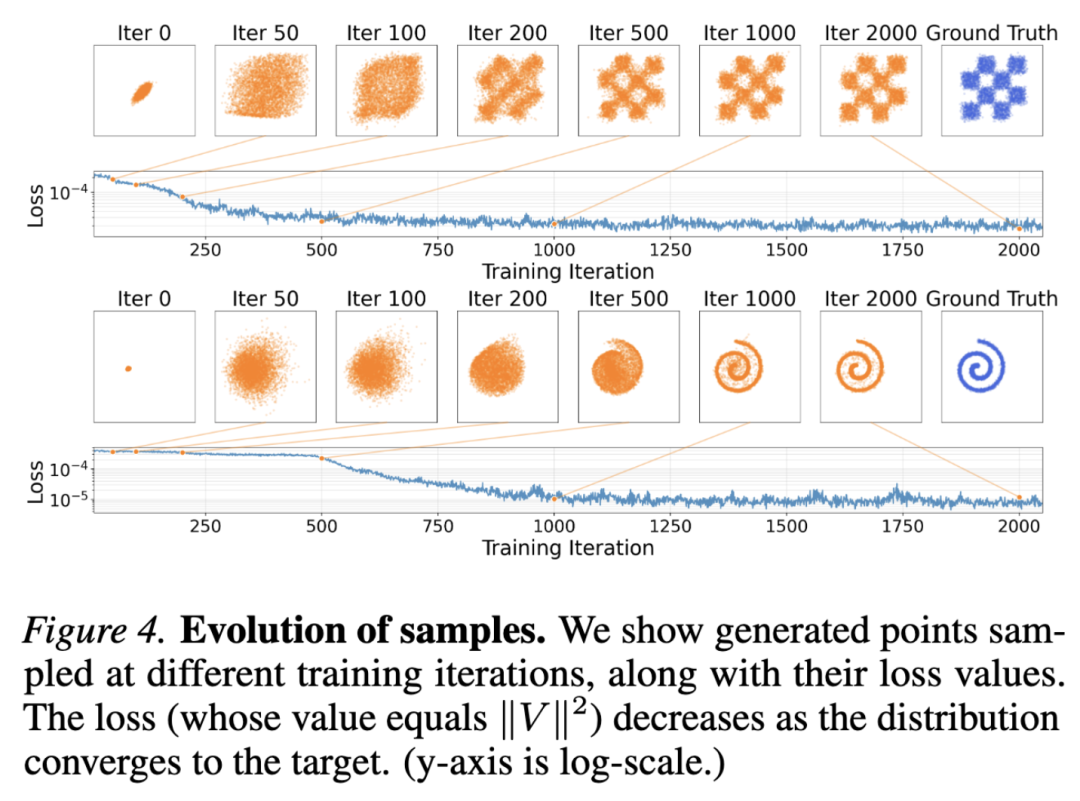
Evolution of Samples. Figure 4 shows the training process on two 2D cases. A small MLP generator is trained. As the generated distribution converges to the target, the loss (whose value equals ) decreases. This aligns with this paper's motivation that reducing drift and pushing toward equilibrium will approximately produce .

ImageNet Experiments

This paper's model is evaluated on ImageNet . Ablation studies use the B/2 model on the SD-VAE latent space, trained for 100 epochs. The drift loss is in the feature space computed by a latent-MAE encoder. This paper reports FID for 50K generated images. This paper analyzes the results as follows.

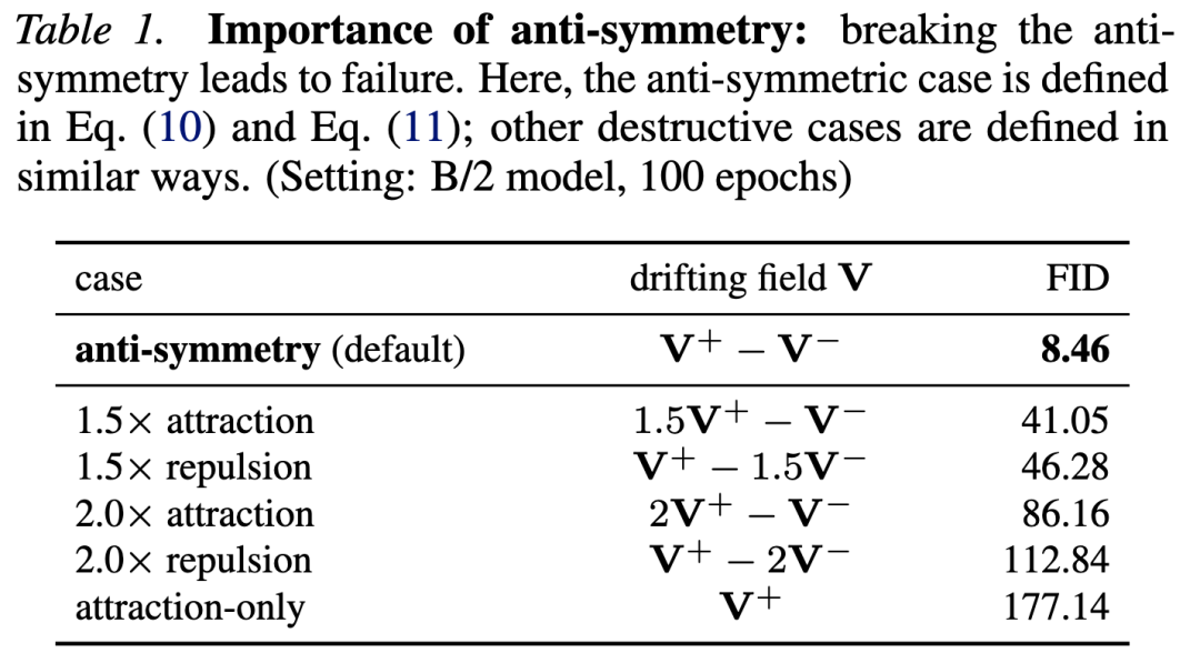
Anti-symmetry. This paper's derivation of equilibrium requires the drift field to be antisymmetric; see formula (3). In Table 1, this paper conducts an ablation study where this antisymmetry is intentionally broken. The antisymmetric case (this paper's default setting for ablation) performs well, while other cases suffer catastrophic failure. Intuitively, for a sample , when and match, this paper expects the attraction from to be canceled by the repulsion from . This balance cannot be achieved in the ablated cases.

Assignment of Positive and Negative Samples. Our method samples positive and negative samples to estimate (see Algorithm 1). In Table 2, we investigate the impact of and under a fixed epoch and fixed batch size.

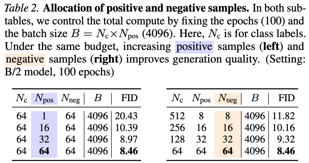
Table 2 shows that using larger and is beneficial. A larger sample size is expected to improve the accuracy of estimating , thereby enhancing generation quality. This observation aligns with results in contrastive learning, where larger sample sets improve representation learning.

Feature Space for Drifting. Our model computes the drift loss in a feature space. Table 3 compares feature encoders. Using publicly available pretrained encoders from SimCLR and MoCo v2, our method achieves promising results.

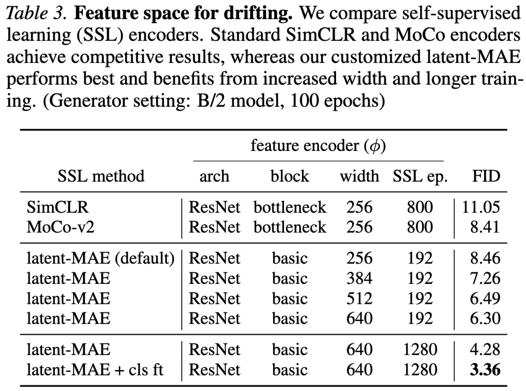
These standard encoders operate in the pixel domain, which requires running the VAE decoder during training. To circumvent this, we directly pretrain a ResNet-style model with an MAE objective on the latent space. This “latent-MAE” yields a strong performing feature space (Table 3). Increasing both the width of the MAE encoder and the number of pretraining epochs improves generation quality; fine-tuning it with a classifier (‘cls ft’) further enhances results to 3.36 FID.

The comparisons in Table 3 indicate that the quality of the feature encoder plays a crucial role. We hypothesize that this is because our method relies on a kernel function (see Eq. 12) to measure sample similarity. Samples that are closer in the feature space typically produce stronger drifts, providing richer training signals. This objective aligns with the motivations of self-supervised learning. A powerful feature encoder reduces the occurrence of nearly “flat” kernels (i.e., vanishes because all samples are far apart).

On the other hand, without a feature encoder, we cannot make the method work on ImageNet. In such cases, even with a latent VAE, the kernel function may fail to effectively describe similarity. We leave further investigation of this limitation to future work.

System-level Comparisons. Beyond ablation settings, we train stronger variants and summarize them in Table 4. Comparisons with previous methods are presented in Table 5.

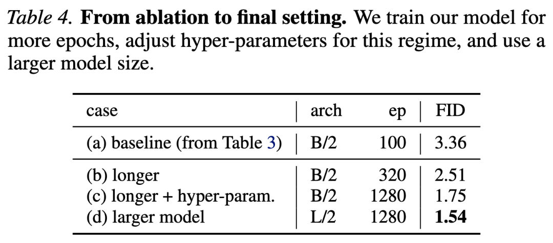
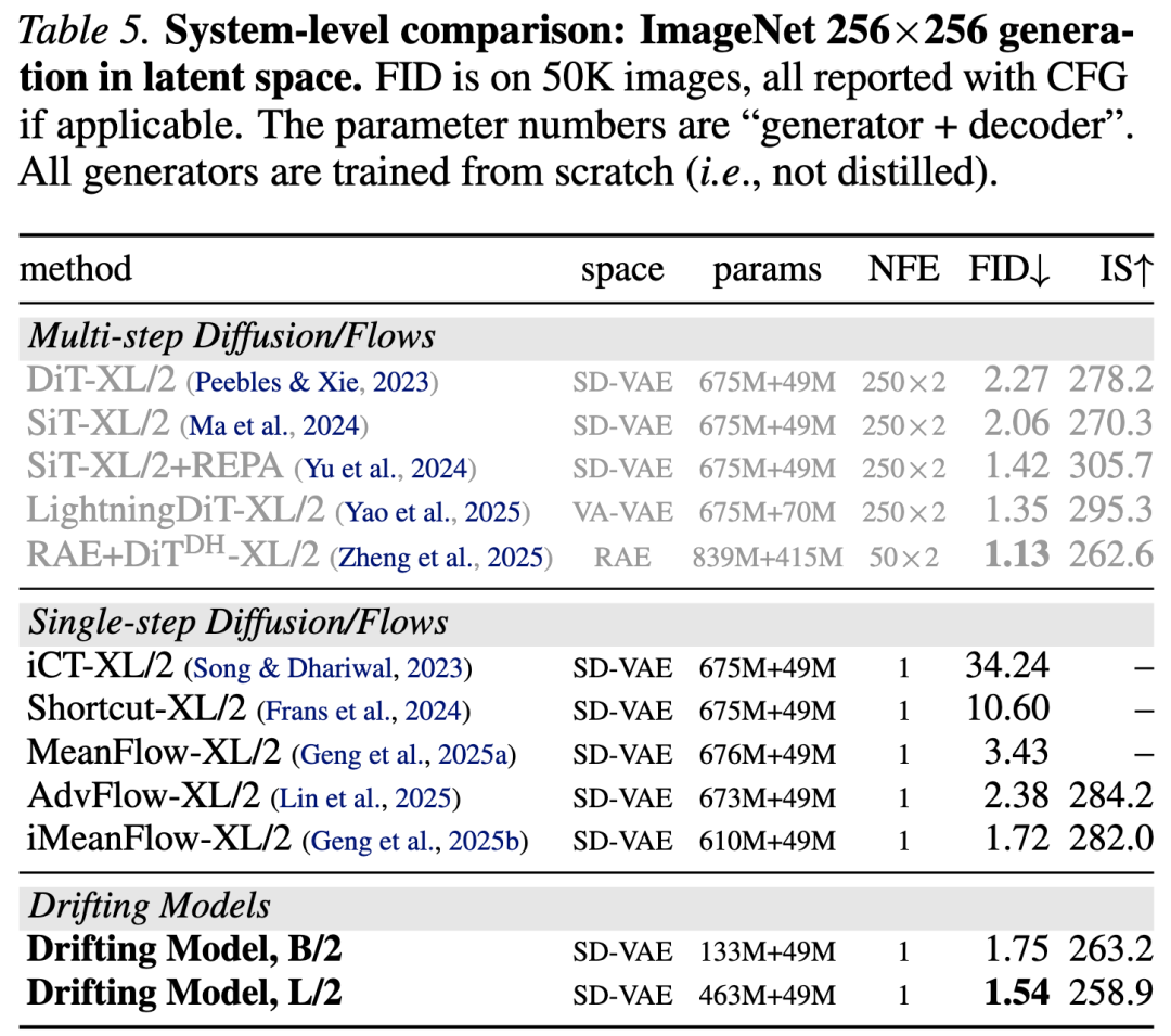
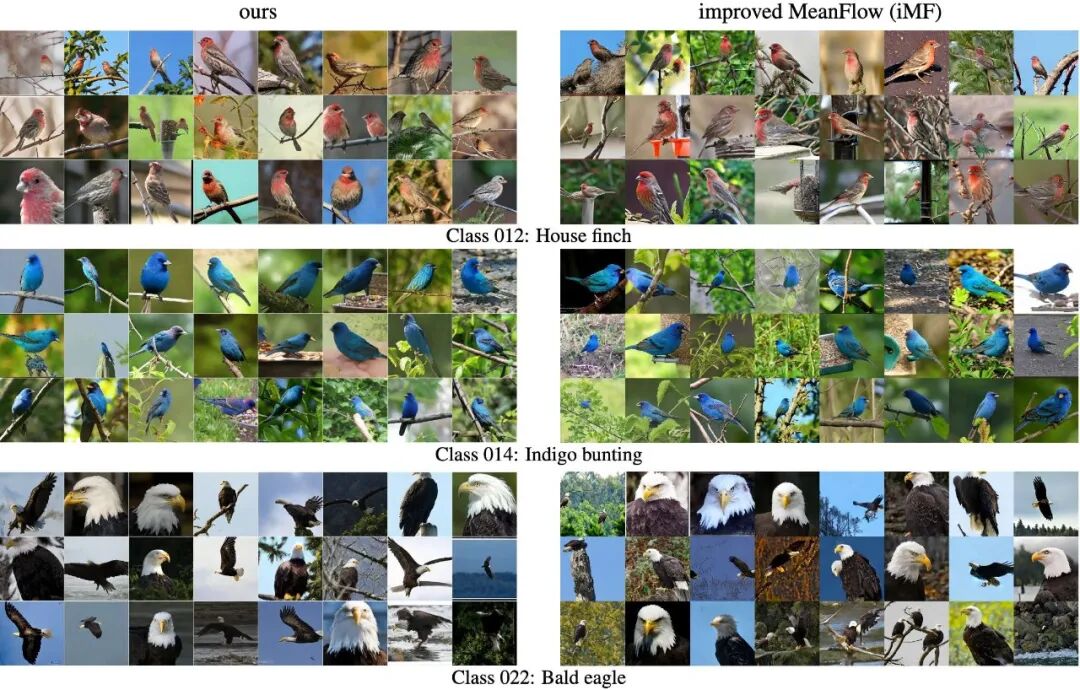
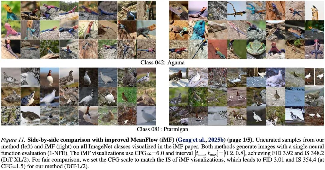
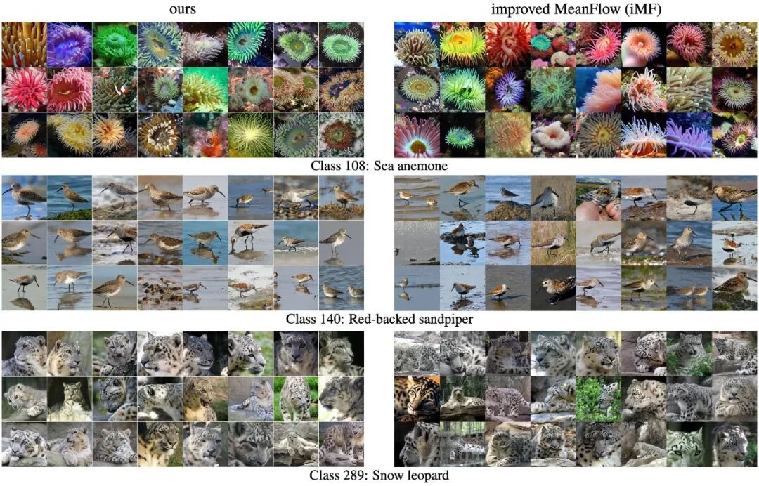
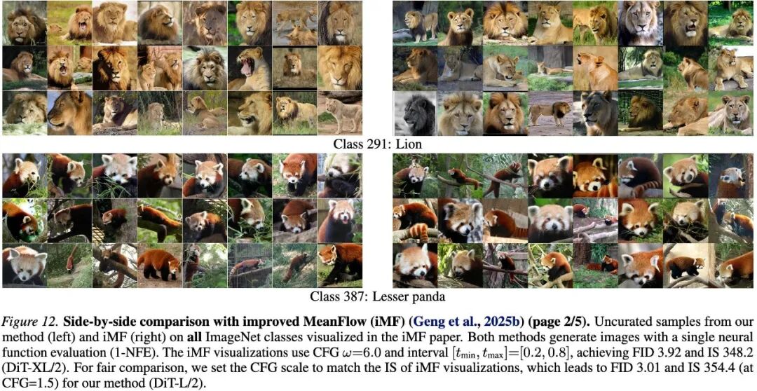
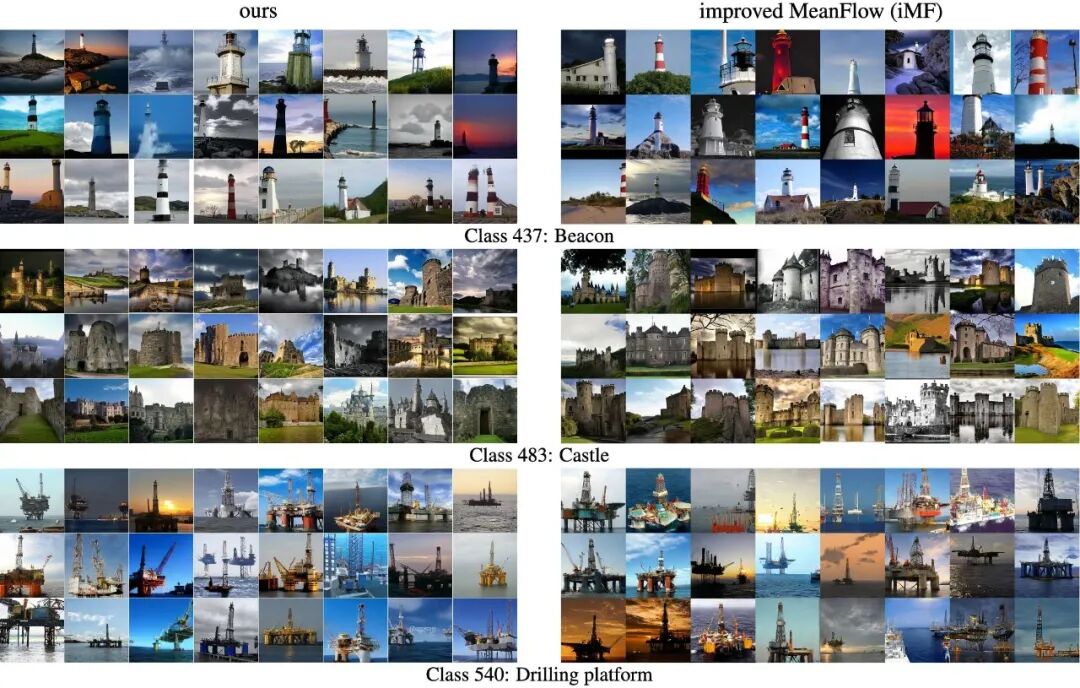
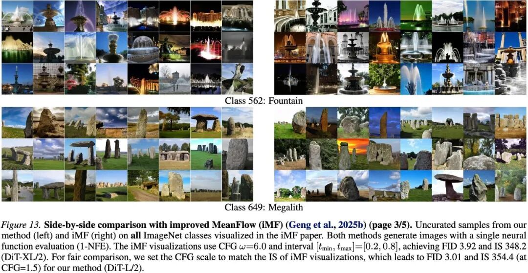
Our method achieves 1.54 FID through native 1-NFE generation. It outperforms all previous 1-NFE methods, which are primarily based on approximating diffusion/flow trajectories. Notably, our Base-sized model is comparable to previous XL-sized models. Our best model (FID 1.54) uses a CFG scale of 1.0, which corresponds to “no CFG” in diffusion models. Our CFG formulation demonstrates an ID and IS trade-off, similar to standard CFG. Additionally, Figs. 11-15 show side-by-side comparisons with improved MeanFlow (iMF), a recent state-of-the-art single-step generation method.

Pixel-space Generation. Our method can naturally operate without a latent VAE, i.e., the generator directly produces images in . The feature encoder is applied to the generated images to compute the drift loss. We adopt a configuration similar to the latent variant; implementation details are provided in Appendix A.

Table 6 compares different pixel-space generators. Our single-step, pixel-space method achieves 1.61 FID, outperforming or matching previous multi-step methods. Compared to other single-step pixel-space methods (GANs), our method achieves 1.61 FID using only 87G FLOPs; in contrast, StyleGAN-XL produces 2.30 FID with 1574G FLOPs.

Robot Control Experiments

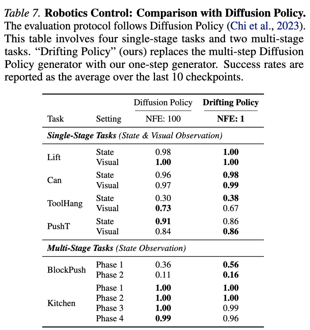
Beyond image generation, we further evaluate our method on robot control. Our experimental design and protocols follow Diffusion Policy. The core of Diffusion Policy is a multi-step, diffusion-based generator; we replace it with our single-step Drifting Model. We compute the drift loss directly on the raw representations of control without using a feature space. The results are shown in Table 7 below. Our 1-NFE model matches or exceeds the state-of-the-art Diffusion Policy using 100 NFEs. This comparison suggests that drift models can serve as a promising generative approach across different domains.

Discussion and Conclusion

We introduce Drifting Models, a new paradigm for generative modeling. The core idea is to model the evolution of the forward distribution during training. This allows us to focus on the update rule, i.e., , during iterative training. This contrasts with diffusion/flow models, which perform iterative updates during inference. Our method naturally performs single-step inference.

Given that our methodology is fundamentally different, many open questions remain. For example, while we demonstrate , the converse does not generally hold in theory. Although our designed performs well empirically, it is unclear under what conditions leads to .

From a practical perspective, while we demonstrate effective instantiations of drift modeling, many of our design decisions may still be suboptimal. For instance, the design of the drift field and its kernel, the feature encoder, and the generator architecture remain to be explored in future work.

From a broader perspective, our work reframes iterative neural network training as a distribution evolution mechanism, in contrast to the differential equations underlying diffusion/flow models. We hope this perspective inspires exploration of other implementations of this mechanism in future work.

References

[1] Generative Modeling via Drifting